Persistent Structures: Key to 2000x Speedup in Neon’s WAL Indexing
2000x Speedup in Neon's WAL Indexing
Neon is a serverless Postgres system that separates storage from compute, providing users with all the customary Postgres features and more, including usage-based billing, autoscaling, database branching, and point-in-time recovery.
We previously provided a comprehensive overview of our storage engine architecture, which enables us to deliver these features. In this article, we elaborate on the read path of the system (the code executed during a read request) and introduce a new data structure that speeds up the storage system’s search for WAL (Write-Ahead Log) by 70 to 2000x compared to our previous non-trivial data structure.
The read path and the big indexing problem
The problem we need to solve is simple: “For a given point in 2D space, draw a line downward and return the first rectangle the line encounters”. Why is Neon solving this problem? And is it that hard? Let’s step back.
As explained in previous articles, the Neon storage system needs to serve historical requests. The storage engine answers GetPage(key, LSN) queries by searching for the requested data in “image” and “delta” layers. The key and LSN are numerical values, with the LSN value representing a point in time.
To answer GetPage(key, LSN) queries, the storage system needs to reconstruct the requested page by applying WAL (Write-Ahead Log) records to a recent page image. But first the storage system needs to find where the WAL for the requested data is stored. This is the problem we’re concerned with in this blog post.
Neon stores WAL and materialized pages in “delta” and “image” layers, respectively (see diagram). The black rectangles are image layers, which contain all the values for a given range of keys at a given time. The tall gray rectangles are delta layers, which only contain all the updates that happened inside a given rectangle in the key-LSN space. The red dots represent seven different historical read queries, and the arrows that extend down from them represent the search path to find the requested layer.
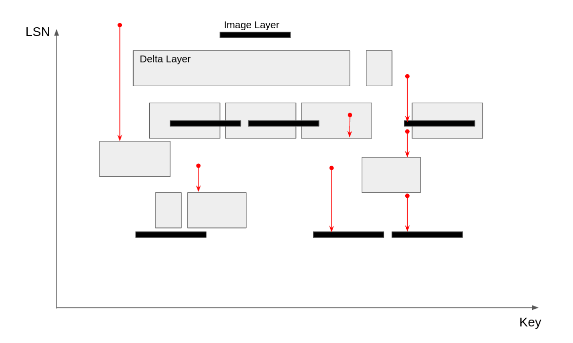
If the first layer encountered is an image layer, we can simply read out the value for the given key from the image layer and return it. But if we hit a delta layer, we need to collect the updates it contains, and continue searching below until we hit an image layer. At that point, we have a tuple (Value, Vec<Update>), and we can use the Write-Ahead Log (WAL) redo process to reconstruct the requested data.
So, that’s why Neon is solving problems with lines and rectangles. To reiterate: “For a given point, draw a line downward and return the first rectangle the line encounters”. How hard can it be? Let’s see.
Failed attempt 1: Just dump it all in a Vec
We can put all the layers in a Vec, and iterate over them until we find the right one. But this O(N) solution won’t work. It’s too slow. We need a really fast solution because we call this search procedure on every request to a storage system, and we get a lot of requests. Think about a single SQL query, which might process gigabytes of data to find the answer. Since the page size in Neon is 8KB, getting 1GB of data means sending 125000 GetPage requests. If all of those take a microsecond, that adds up to 0.125 seconds, which is good, but if they take seconds… it’s a non-starter. The number of layers is in the tens of millions (and likely more in the future), so any O(N) solution is too slow.
Failed attempt 2: Spatial data structure
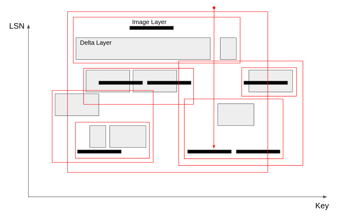
An R-Tree is a canonical data structure for querying rectangles. It sort of groups rectangles into bigger ones, allowing you to search faster, but it’s not ideal for what we want. It’s meant for point queries. It can quickly find the rectangle that contains the point by searching hierarchically and ruling out a large number of rectangles at a time. But what if the point is not contained in a rectangle? In this case, we want the first rectangle below the point. As shown in the diagram, all that grouping doesn’t help. We still need to traverse the tree all the way down in some cases, which means our worst case is O(N). This would be fine if it wasn’t so easy to trigger in practice. But it’s slow, and it is a shame for a database system dealing with disk, s3, network latency, etc., to struggle with in-memory search problems. This search should not even show up on our flame graphs.
Failed attempt 3: Segment tree
You can skip this section if you want, but any competitive programmer reading this post will be screaming, ‘SEGMENT TREEES!!!’ So, we have to address them. Yes, segment trees are the canonical data structure for range queries but they’re much more popular in 5-hour contests than they are in real-world systems. Why is that? Wait, what’s a segment tree?
A segment tree (different from an interval tree) is a materialized divide-and-conquer solution. Split the space in half, store something about each half, and store a summary in the root. What that “something” is depends on the situation, which makes segment trees applicable to a large variety of problems.
To familiarize ourselves with segment trees, let’s do a completely unrelated practice problem: Given an array of N integers, answer the following queries:
- update(key, val): change the number at key to val in O(log N)
- get_min(begin, end): return the smallest value in range [begin, end) in O(log N)
This is also known as the “Range Maximum Problem”. Segment trees solve it quite well, which is why they are sometimes categorized as a “range query” technique. Here’s how the solution works:
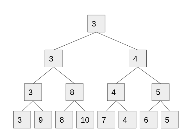
First we recursively split the list in half, effectively organizing it into a binary tree, where the leafs are the elements. Inside each non-leaf node, we store the minimum value for all its children (see diagram). Now, to implement update, we change the value of the leaf and propagate the changes up the tree. To answer a query, we descend down from the root to find O(log N) nodes that cover our range, taking their minimum without descending all the way down.
So, we saw how to materialize a divide-and-conquer solution into a segment tree for the Range Minimum Query problem. But how do we solve the Neon Layer Map search problem? It’s two dimensional!! Which way do we “divide” the problem? In general, what’s a good way to subdivide a 2D space for divide-and-conquer solutions?
There’s a right way, but let’s first rule out the two most tempting ways to subdivide the space: split into four quadrants, or split in halffour different ways, as shown in the following diragrams, respectively:
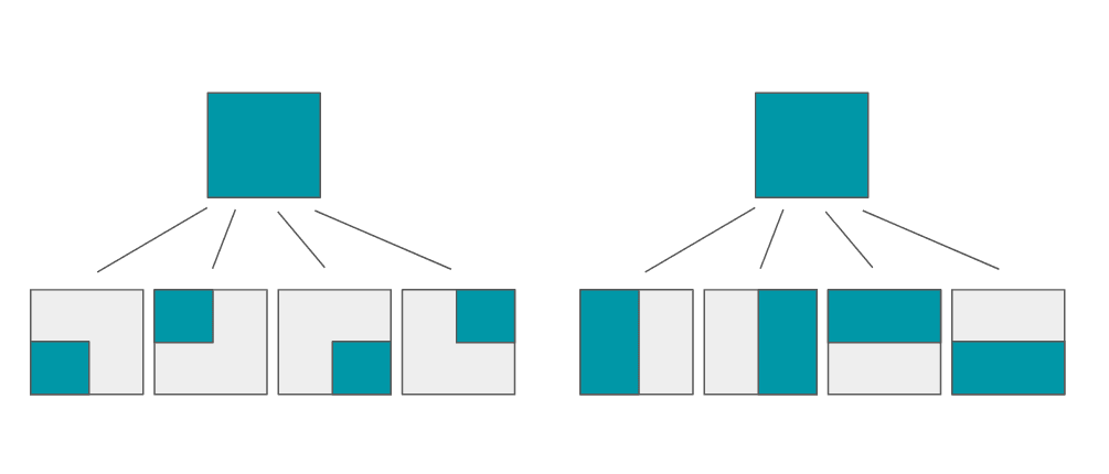
The first approach doesn’t work because it doesn’t allow O(log N) querying (an exercise left for the reader). The second approach would require O(N^2) storage (hint), so we don’t even have time to construct it.
The one good way (that I know of) to use segment trees in two dimensions is to split in the first dimension only, and then put an entire segment tree at each node, which splits in the second dimension, effectively creating a segment tree of segment trees. In this arrangement, the outer segment tree directs you to a set of inner segment trees whose union can give you the result. Since we’re now querying O(log MAX_KEY) segment trees, and each query takes O(log MAX_LSN), our total query runtime is O(log MAX_KEY * log MAX_LSN).
Even though this runtime is better than an R-Tree, this approach has two flaws:
- MAX_KEY and MAX_LSN are very large numbers. We’d rather be talking in O(log N), where N is the number of layers. In cases like this, usually Coordinate Compression can help, but it requires up-front knowledge of all the queries. We really need a balancing data structure. It’s possible to balance 1D segment trees (and maybe 2D, too?), but…
- This is very complicated to implement already, and if we add balancing and “lazy propagation” (yet another advanced technique that’s necessary for fast updates), we would blow our complexity budget. Remember, even though I’m only talking about the point/line search query here, it doesn’t mean it’s the only real-world requirement of this data structure. It also needs to efficiently iterate and aggregate things for other purposes, which is non-trivial to implement on top of the segment tree. Things are complex already!
Rust Persistent Data Structures (RPDS) to the rescue
We were ready to bite the bullet and roll out our own balanced 2D segment tree with lazy propagation until we discovered a simpler and faster approach which outperformed the R-Tree by 70x on current real databases, and 2000x on synthetic tests with a projected larger database size. The secret sauce: the rpds (Rust Persistent Data Structures) crate.
What are persistent (a.k.a. immutable) data structures? It’s an advanced technique, but very simple in retrospect: take any tree-based data structure, make it copy-on-write, and now you can query any past state of the data structure. See this diagram, for example:
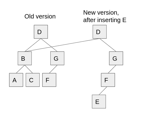
When we add the value E, we don’t mutate node F to add a child. Instead, we copy it and add a child to the copy. Then, we attach this new F node to a copy of it’s parent G, and attach that new G to a copy of the root, D. Now, we have two roots, and we can use the old root to query a past state, or use the new root to query the current state.
Why is this useful to us? Because if we have a tree-based data structure that efficiently solves the latest-only problem (querying with latest LSN), we can just convert that data structure into a persistent one, and time travel back into the past when we need to answer queries about historical LSNs.
So, let’s look at the latest-only problem (see diagram). Can we solve it efficiently with a tree-based data structure?
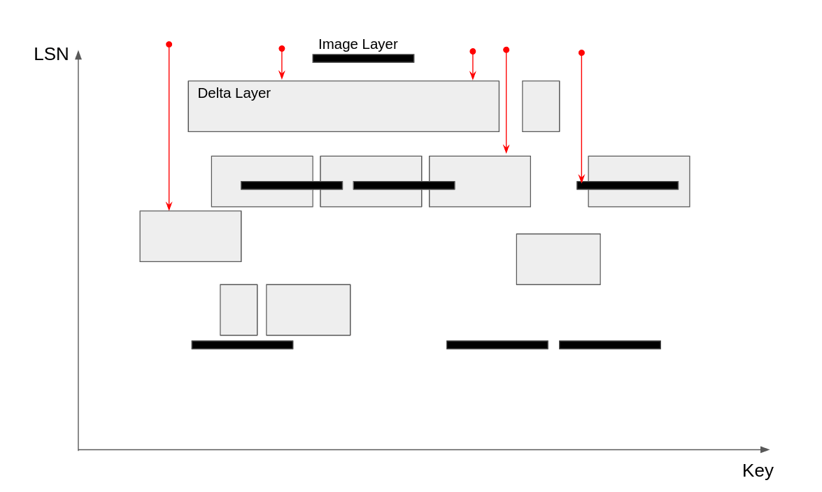
Yes! We can precompute the answer for every single key, take all the points where the answer changes as we look from left to right, and store them in a BST (binary search tree). We call this BST the “Layer Coverage” for a given LSN. The following diagram shows the layer coverage for the latest LSN:
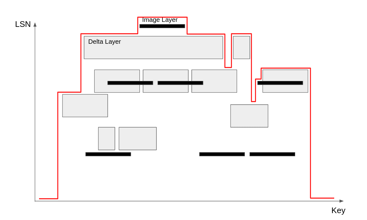
The layer coverage can be queried in O(log N) to answer latest-only queries. In Rust we can use the .range(..K).next_back() method (C++ programmers might be more familiar with the equivalent lower_bound() method).
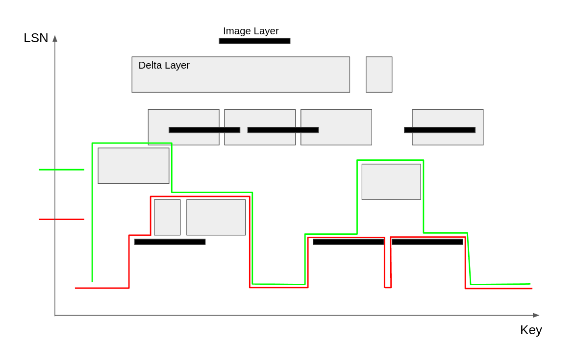
But to answer historical queries in O(log N), we need to upgrade this BST to a persistent BST, and correctly order the insertions to it. We need to build it starting from the bottom so that past versions of the tree correspond to different LSNs. Here’s a step-by-step visualization of the layer coverage, built from bottom to top. The red line shows the layer coverage after inserting the first 5 layers, in sorted order.
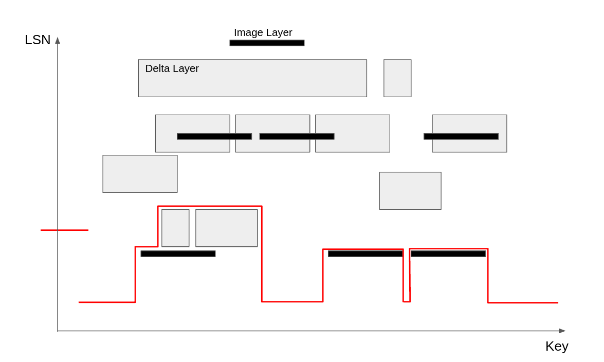
The green line shows the layer coverage after inserting 2 more layers. Remember, this is a copy-on-write data structure, so we still have the red layer coverage if we want to query that point in the past.
And so on…
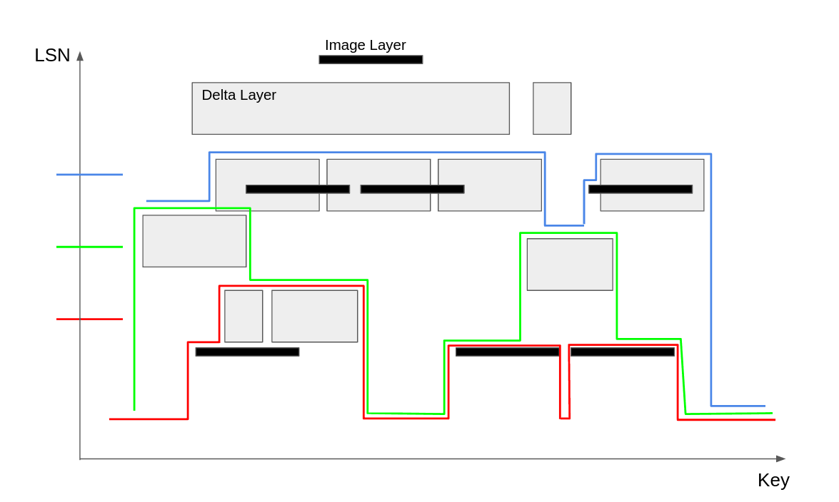
At the end, we have a layer coverage for every single LSN. At first, it might seem like the construction and space cost is O(N^2), but it’s actually O(N * log N), and here’s why:
- Every layer accounts for at most two insertions: one for the top-left corner, and one for the top-right corner. So, in total, we insert O(N) things.
- Every layer accounts for potentially many more deletions, but the total number of deletions is not more than the total number of insertions. So, in total, we remove O(N) things.
- Insertion is O(log N). So, in total, we spend O(N * log N) time inserting.
- The space complexity can’t be more than the construction time complexity, so it’s also O(N * log N).
Conclusion
Our new layer map data structure is way faster than we need it to be, and the bottleneck is just 2 BST lookups, an Arc::clone(), and a few other small things. The only way to further improve this for our purposes is to simplify it.
Overall it was a 2000 line PR with more nuance than can fit in a blog post (the layer map supports other queries too), and the code can be found here. The microbenchmarks are also open-source, and you’re welcome to beat our solution. It’s possible we’ve missed a much simpler solution, and we’d rather know sooner than later 🙂
Big thanks to the maintainers of the rpds crate, which does most of the heavy lifting for us. There are more popular persistent data structure libraries in Rust, but this one deserves a lot more credit for its clean API, correct results (!!!), and more than good enough performance.
I’ll end with a quote by Dan Luu on the “Purely Functional Data Structures” book, which explains among other things, persistent data structures: “… Fun to work through, but, unlike the other algorithms and data structures books, I’ve yet to be able to apply anything from this book to a problem domain where performance really matters.” Well, we now have at least one such example.
Thanks to Predrag Gruevski for his feedback on drafts of this post. All mistakes are mine alone.

